Constrained Multi-Vehicle Routing Algorithm

A heuristic algorithm for computing multi-vehicle package delivery routes.

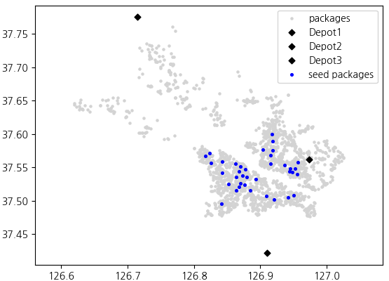
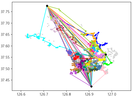
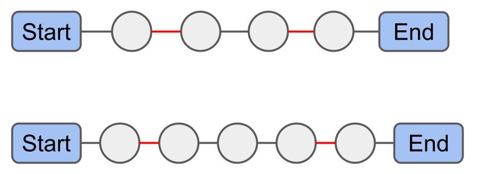
Algorithm Visualization

Input: 3 depots, 2205 packages, 37 vehicles with a total capacity of 1805.

Output: 37 routes, a total of 1805 packages delivered.

Key Highlights

Won 2nd place (out of 103 teams) in the 2022 CJ Logistics Future Technology Challenge.
Achieved the maximum possible delivery count on the competition dataset (37 vehicles, 1,805 packages) using only 73.5% of the vehicle resources and satisfying constraints on vehicle capacity, travel distances, and per-package delivery time windows.
Decreased runtime by 20% using multi-threading, while maintaining deterministic results.

Objective

The goal of the algorithm is to produce package delivery routes for all vehicles while satisfying the constraints below.

Vehicle Constraints

Fixed start and end depot, where start depot $ \neq $ end depot.
Vehicle-specific capacity (given as an integer, e.g. 50).
Vehicle-specific working hours (e.g. 6/20/2022 00:00 ~ 6/20/2022 05:00).
Maximum daily travel distance (110km).
Fixed traveling speed (40km/h).

Package Constraints

Package-specific volume (same unit as vehicle capacity, given as an integer).
Package-specific drop-off time window (e.g. 6/20/2022 01:00 ~ 6/20/2022 02:00).
Package-specific unloading-from-vehicle time (e.g. 2 min.).
Some packages require a specific vehicle (e.g. package A00012 can only be delivered by vehicle #11).
Some packages can only be delivered by ‘small’ trucks. Each vehicle is classified as either ‘big’ or ‘small’.

Methodology

The algorithm consists of two stages: insertion heuristic and local search.

First, the insertion heuristic constructs tentative routes that satisfy all vehicle and package constraints. Then, local search iteratively improves the routes by making small intra/inter-route modifications.

Insertion Heuristic

The insertion heuristic consists of three steps: seed selection, seed insertion, and iterative insertion.

Seed selection: The first packages inserted into each route are called 'seeds'. Seed selection is an important step because the insertion heuristic's results can vary greatly by how these seeds are selected.

This algorithm follows Savelsbergh's[1] method to select seeds based on the distribution density of the packages' drop-off locations.

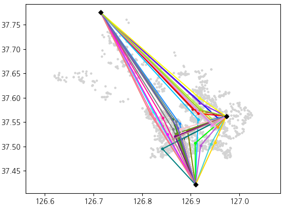
Seed insertion: Seeds are inserted into each route using the "look-ahead heuristic" (a.k.a. 'regret')[1]. Regret stands for the cost difference between the best and second-best choices. Prioritizing the insertion of packages with the biggest regret can be interpreted as trying to minimize the potential future loss when the package's best insertion choice is no longer available.

The cost function used to calculate the best choice and second-best choice is simply (distance from start depot to package drop-off site) + (distance from package drop-off site to end depot).

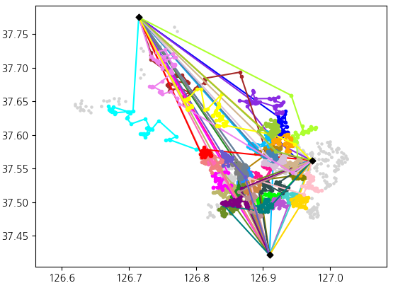
Iterative insertion: The rest of the drop-off sites are inserted into the routes using a modified version of Solomon’s[2] time-window-based insertion heuristic. The modified formulas are as below.

\[c_1 = b_i' - b_i\] \[c_2 = (t_{start} + t_{unload} + t_{end} - c_1 - 2t_{centroid}) \times (p / q)\]

Explanations on each symbol. (Click Me)

Given that a new package $u$ gets inserted into route $r$ right before package $i$

$b_i'$: delayed drop-off time for package $i$ after inserting package $u$
$b_i$: original drop-off time for package $i$ before inserting package $u$
$t_{start}$: travel time from start depot to package $u$ drop-off site
$t_{unload}$: unloading time required by package $u$
$t_{end}$: travel time from package $u$ drop-off site to end depot
$t_{centroid}$ travel time from package $u$ drop-off site to route $r$'s centroid
$p$: profit of package $u$
$q$: volume of package $u$

$c_1$ can be interpreted as the time cost required to add the new package to the route.

$c_2$ can be interpreted as the time cost saved by not having to deliver the new package separately in a new vehicle.

Of all the unrouted packages, the package with the largest $c_2$ should be prioritized, and that package should be inserted at the place that minimizes its $c_1$.

The formula for $c_2$ includes profit/volume ratio $p/q$ because the algorithm should prioritize packages with a higher profit ratio.

The use of a centroid-based penalty $t_{centroid}$ is inspired by Golden[3]. The centroids for each route are updated after every insertion.

The centroid of a route is calculated by averaging the coordinates of the route’s depots and drop-off sites, weighted by their profit/volume ratio. Depots are assumed to have the average profit and volume of all packages in the dataset.

Local Search

Local search iteratively improves the routes by making small intra/inter-route modifications.

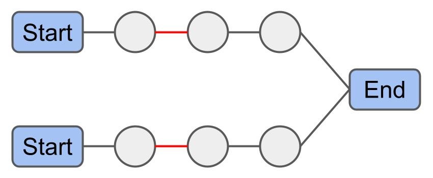
Inspired by Aras[4], Mcnabb[5], and Vansteenwegen[6], the local search operators used in this algorithm are Replacement, Deletion, 1-0 Move, Chain Swap, 1-1 Move, Insertion, and Or-Opt. Detailed descriptions of each operator can be found in Appendix A.

The local search continues until it fails to make any improvement for max_patience number of loops around all the operators, where max_patience is a hyper-parameter.

Multi-threading is applied to a few of the local search operators to speed up the search while maintaining deterministic results. See Appendix B for details.

Results

Below are the results of the algorithm when tested on the dataset from 2022 CJ Logistics Future Technology Challenge. The dataset contains 2200 packages and 37 vehicles with a total capacity of 1805.

Result after insertion heuristic ():

Total number of delivered payloads: 1748
Total time cost: 136h 45m 05s
Total distance cost: 3132.8km
Algorithm runtime: 11.0s

Result after local search ():

Total number of delivered payloads: 1805
Total time cost: 133h 03m 05s
Total distance cost: 2921.3km
Algorithm runtime: 2m 00s

Routes produced by insertion heuristic. — Routes after insertion heuristic is complete.

Routes produced by local search. — Routes after local search is complete.

Limitations and Future Work

Given $n$ packages, the algorithm has a time complexity of $O(n^3)$, making it inefficient for large datasets. For scalability, large datasets should be split into smaller, mutually exclusive subsets of packages and vehicles, and the algorithm should be applied separately to each subset. Future work should explore how such splitting can be done based on geographical regions and random sampling.
Due to the competition’s time limit (1.5 months), the algorithm has only been tested on small variations of the competition dataset. Future work should evaluate the algorithm on a broader set of randomized datasets alongside alternative designs to better justify its design choices.

References

[1] SAVELSBERGH, M. W. P. A parallel insertion heuristic for vehicle routing with side constraints. Statistica Neerlandica, 1990, 44.3: 139-148.

[2] SOLOMON, Marius M. Algorithms for the vehicle routing and scheduling problems with time window constraints. Operations research, 1987, 35.2: 254-265.

[3] GOLDEN, Bruce L.; LEVY, Larry; VOHRA, Rakesh. The orienteering problem. Naval Research Logistics (NRL), 1987, 34.3: 307-318.

[4] ARAS, Necati; AKSEN, Deniz; TEKIN, Mehmet Tuğrul. Selective multi-depot vehicle routing problem with pricing. Transportation Research Part C: Emerging Technologies, 2011, 19.5: 866-884.

[5] MCNABB, Marcus E., et al. Testing local search move operators on the vehicle routing problem with split deliveries and time windows. Computers & Operations Research, 2015, 56: 93-109.

[6] VANSTEENWEGEN, Pieter, et al. A guided local search metaheuristic for the team orienteering problem. European journal of operational research, 2009, 196.1: 118-127.

Appendix A: Local Search Operators

The local search loop consists of Replacement, Deletion, 1-0 Move, Chain Swap, 1-1 Move, Insertion, and Or-Opt. With the exception of the deletion operator, all operators are only performed if they improve the profit and/or efficiency of the routes.

Replacement: Replace a routed package with an unrouted package.

Deletion: From each route, remove at most three packages with the lowest profit/volume ratio, largest distance cost, and longest wait time. By removing the worst packages, this operator creates leeway for packages to move around between routes.

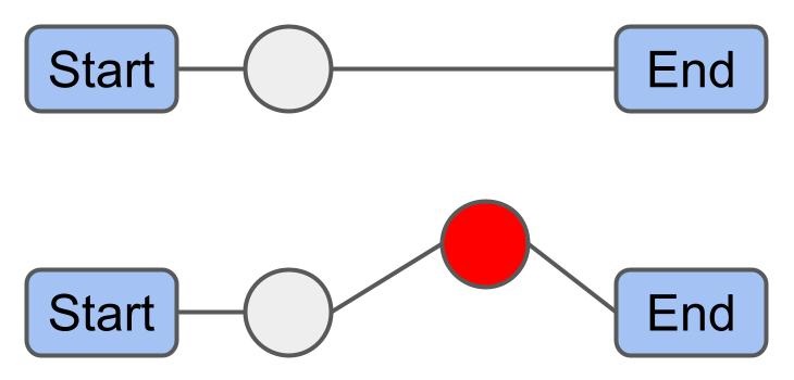
1-0 Move: Remove a package from one route and insert it into another route.

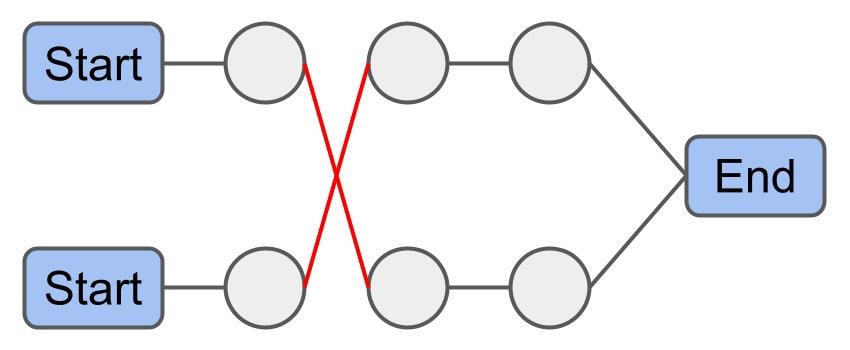
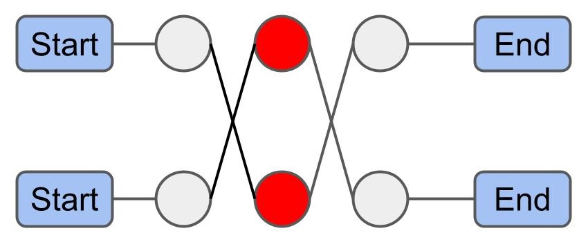
Chain Swap: Given that routes $ r_x $ and $ r_y $ share the same end depot, swap all packages in $ r_x $ starting from its $i^{th}$ package with all packages of $ r_y $ starting from its $j^{th}$ package.

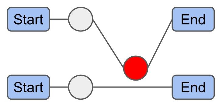
1-1 Move: Exchange a package from one route with a package from another route.

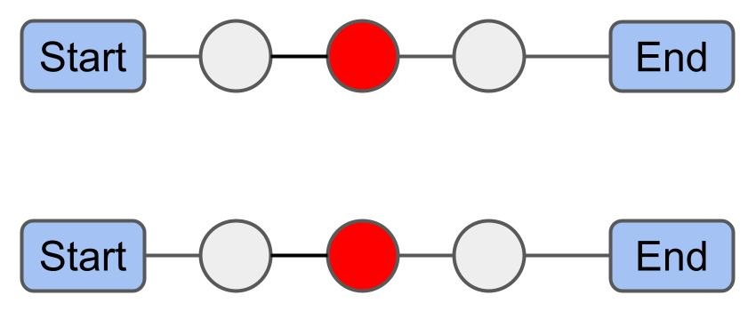
Insertion: Insert unrouted packages into routes by using the insertion heuristic. Ignore centroid-based penalty.

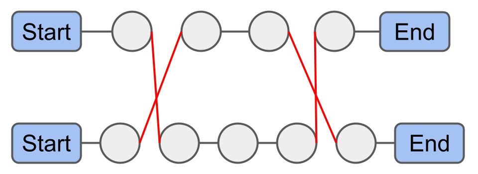
Or-Opt: swap $i^{th}$ to $(i+n)^{th}$ packages of route $ r_x $ with $j^{th}$ to $(j+m)^{th}$ packages of route $ r_y $.

Appendix B: Multi-threading with Deterministic Results

Inter-route local search operators (e.g. 1-0 Move, 1-1 Move, and Or-Opt) move and swap packages between two routes. These operators all have a double-nested loop structure shown below.

for (int i = 0; i < routes.size(); ++i) {
	for (int j = i+1; j < routes.size(); ++j) {
		performLocalSearchOperator(routes[i], routes[j]);
	}
}

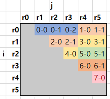
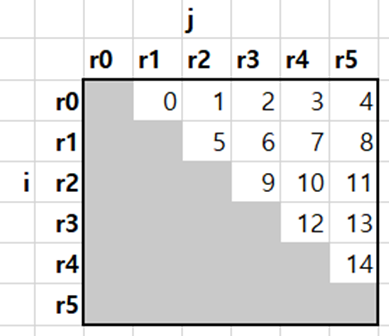
Given 6 routes $r_0$ through $r_5$, the above double-nested loop can be illustrated as . The number in each cell indicates the order in which a single-thread single-thread program would execute the local search operators on these routes.

From , it can be seen that each cell is dependent on the cell to its left. For example, the result of cell 2 (performing the local search between $r_0$ and $r_3$) depends on the result of cell 1 (which performs local search between $r_0$ and $r_2$). This is because both cells share the same $r_0$. Likewise, we can see that each cell is dependent on the cell above. For example, the result of cell 10 (performing the local search between $r_2$ and $r_4$) depends on the result of cell 7 (which performs local search between $r_1$ and $r_4$), because both cells share the same $r_4$.

To get deterministic results, the multi-thread execution must maintain the same dependencies as the single-thread execution. illustrates how multiple threads can split the workload while maintaining such dependencies. The number in each cell represents (thread id)-(execution order within the thread) and the threads that are executed simultaneously are given the same color. Each thread begins when the thread to its left and above has both completed executing.

Hence, similar to an assembly pipeline, when thread 0 finishes executing, threads 1 and 2 begin simultaneously. When threads 1 and 2 both finish executing, then threads 3 and 4 begin simultaneously. Given a larger number of routes, this pattern of execution can be applied using a larger number of threads to improve efficiency.

← Back to ‘Projects’

Junhwan Kim